Proteomics by mass spectrometry: what is inside a raw file

写作说明

本文由 DeepSeek-Flash 生成，尚未经过人工校对，可能存在事实、数字或表述上的错误，请以原始文献、仪器手册和官方文档为准。

文中的所有图表都由本文的 R 代码在渲染时生成，其中的数值是为说明概念而模拟的，不代表任何真实仪器、样本或数据集。软件包名称与文件格式的描述基于公开文档，但版本演进很快，实际使用时请以对应版本的文档为准。

蛋白质组学最容易被误解的一点是：很多人以为”测一个蛋白”就是仪器直接报告一个浓度。实际上，基于质谱的蛋白质组学测的是肽段的质荷比和信号强度，蛋白是从这些肽段反推出来的。所以一个 .raw 文件里并没有”蛋白”这个字段，只有成千上万张质谱图，以及每张图属于哪一次扫描、在什么时间、用什么参数采集。

这篇文章按数据实际流动的顺序展开：

1. 蛋白质组学要回答什么问题，为什么难；
2. 一台 LC-MS/MS 里到底发生了什么；
3. 原始数据里存了哪些字段；
4. DDA、DIA、PRM 三种采集策略；
5. 厂商封闭格式与开放格式（mzML 等）的架构差别；
6. 用 Python 和 R 把数据读进来；
7. 从谱图到蛋白表：搜库、FDR、蛋白推断、定量、缺失值；
8. 除了基于质谱的方法，还有哪些蛋白质组学路线，各自能回答什么。

目标是写成一份可以按图索骥的技术报告。

1. 蛋白质组学测的是什么，为什么难

基因组是一份稳定的序列，转录组是”此刻在转录什么”，而蛋白质组是此刻真正在执行功能的分子。三者之间并不是简单的一一映射：

• 一个基因可以产生多种蛋白质形式（proteoform）：可变剪接、蛋白酶切、信号肽去除；
• 蛋白丰度与 mRNA 丰度只有中等相关（常见报道在 0.4–0.6 之间），因为翻译效率和降解速率不同；
• 蛋白会被修饰（磷酸化、乙酰化、泛素化、糖基化、氧化），修饰状态往往才是功能开关；
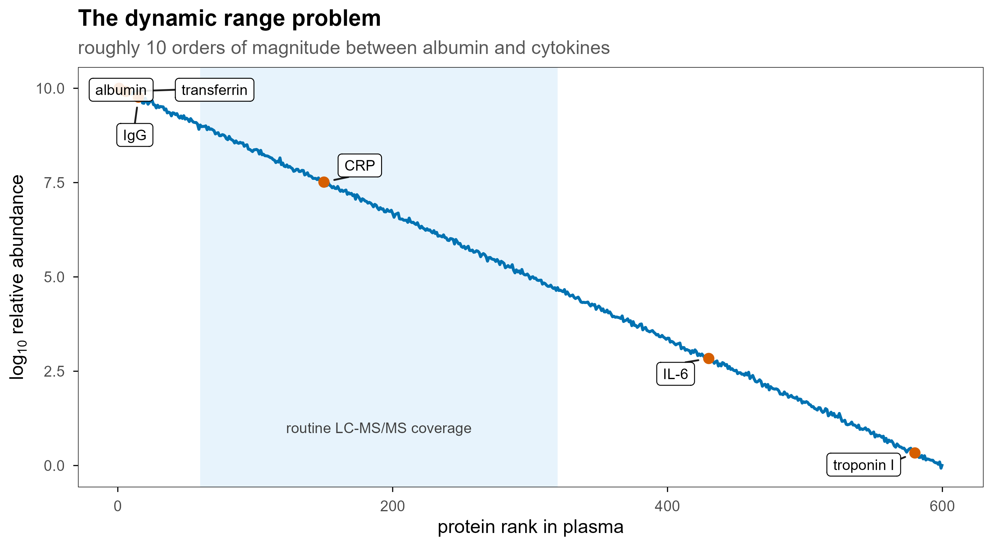
• 蛋白丰度的动态范围极大：血浆中白蛋白与低丰度细胞因子之间可以相差 10 个数量级。

set.seed(42)
ab <- data.frame(rank = 1:600)
ab$log_ab <- 10 - 10 * (ab$rank - 1) / 599 + rnorm(nrow(ab), 0, 0.04)

mark <- data.frame(
  protein = c("albumin", "transferrin", "IgG", "CRP", "IL-6", "troponin I"),
  rank = c(1, 6, 15, 150, 430, 580)
)
mark$log_ab <- 10 - 10 * (mark$rank - 1) / 599

set.seed(1)
ggplot(ab, aes(rank, log_ab)) +
  annotate("rect", xmin = 60, xmax = 320, ymin = -Inf, ymax = Inf,
           fill = blog_pal[["sky"]], alpha = 0.14) +
  annotate("text", x = 190, y = 1.0, label = "routine LC-MS/MS coverage",
           size = 3, colour = "grey25") +
  geom_line(colour = blog_pal[["blue"]], linewidth = 0.8) +
  geom_point(data = mark, colour = blog_pal[["vermillion"]], size = 2.4) +
  geom_label_repel(
    data = mark, aes(label = protein), size = 3,
    fill = "white", alpha = 0.88, label.size = 0.2,
    min.segment.length = 0, box.padding = 0.45, point.padding = 0.35,
    max.overlaps = Inf
  ) +
  labs(
    x = "protein rank in plasma", y = expression(log[10]~"relative abundance"),
    title = "The dynamic range problem",
    subtitle = "roughly 10 orders of magnitude between albumin and cytokines"
  )

Figure 1: 血浆蛋白的丰度横跨约 10 个数量级。质谱一次进样能覆盖的主要是中间那一段，最两端通常需要去除高丰度蛋白或富集低丰度蛋白。

把这件事翻译成数据语言，就是三个不同层次的问题：

层次	问题	数据产物
鉴定（identification）	样本里有哪些肽段和蛋白	PSM 表、peptide 表、protein 表
定量（quantification）	每个蛋白在不同样本里有多少	强度矩阵、比值、差异检验结果
状态（state）	修饰位点、互作、定位、结构	位点表、互作网络、交联对、HDX 曲线

后面所有的文件格式和分析步骤，都是为这三层服务。

2. 一台 LC-MS/MS 里发生了什么

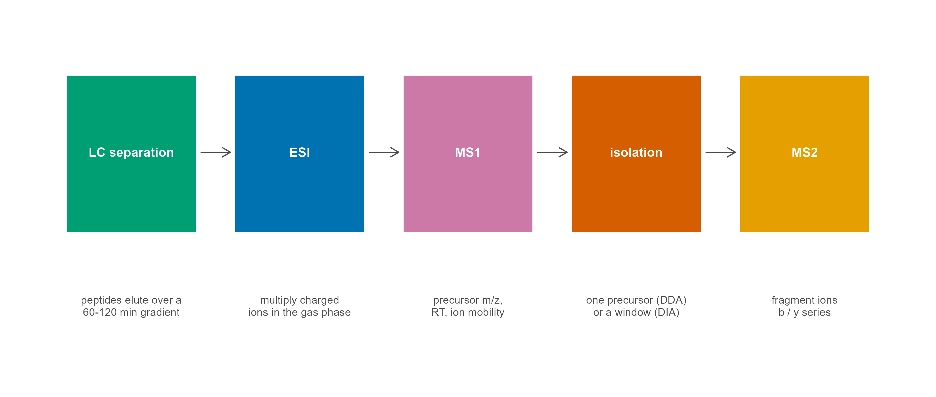
自下而上（bottom-up）蛋白质组学的标准流程是：提取蛋白 → 酶切成肽段 → 液相色谱分离 → 电喷雾离子化 → 质谱测量 → 数据库搜索。之所以先酶切，是因为完整蛋白太大、太难气化和碎裂；胰蛋白酶（trypsin）在 Lys/Arg 之后切割，产生长度和带电性质都比较适合质谱的肽段（常见 7–25 个氨基酸）。

steps <- data.frame(
  x = c(1, 2.75, 4.5, 6.25, 8),
  head = c("LC separation", "ESI", "MS1", "isolation", "MS2"),
  sub = c(
    "peptides elute over a\n60-120 min gradient",
    "multiply charged\nions in the gas phase",
    "precursor m/z,\nRT, ion mobility",
    "one precursor (DDA)\nor a window (DIA)",
    "fragment ions\nb / y series"
  )
)
links <- data.frame(x = steps$x[-nrow(steps)] + 0.72, xend = steps$x[-1] - 0.72)

ggplot() +
  geom_rect(
    data = steps,
    aes(xmin = x - 0.68, xmax = x + 0.68, ymin = 0.42, ymax = 0.90, fill = head),
    colour = "white", linewidth = 0.7
  ) +
  geom_text(data = steps, aes(x, 0.665, label = head),
            colour = "white", fontface = "bold", size = 3.2) +
  geom_text(data = steps, aes(x, 0.20, label = sub),
            size = 2.7, colour = "grey30", lineheight = 0.95) +
  geom_segment(
    data = links, aes(x = x, xend = xend, y = 0.665, yend = 0.665),
    arrow = arrow(length = unit(2.4, "mm")), colour = "grey30", linewidth = 0.4
  ) +
  scale_fill_manual(values = pal[1:5], guide = "none") +
  coord_cartesian(xlim = c(0.15, 8.85), ylim = c(0, 1.05), clip = "off") +
  theme_blog() +
  theme(
    axis.text = element_blank(), axis.title = element_blank(),
    axis.ticks = element_blank(), panel.border = element_blank(),
    legend.position = "none"
  )

Figure 2: 自下而上蛋白质组学的主链路。每一步的产物都是一个可检查的中间文件，这也是排错时最有效的定位顺序。

几个决定数据形态的物理事实：

• 电喷雾（ESI）让肽段带上多个质子，所以同一个肽段会以 2+、3+、4+ 等多个电荷态出现，质荷比不同，但”质量”相同。
• 质量分析器决定分辨率、质量精度和扫描速度。Orbitrap 分辨率高、质量精度好；TOF 扫描快；离子阱便宜；四极杆常作为前级过滤或做 PRM。这些硬件差别直接决定了 mzML 里每条 scan 的元数据。
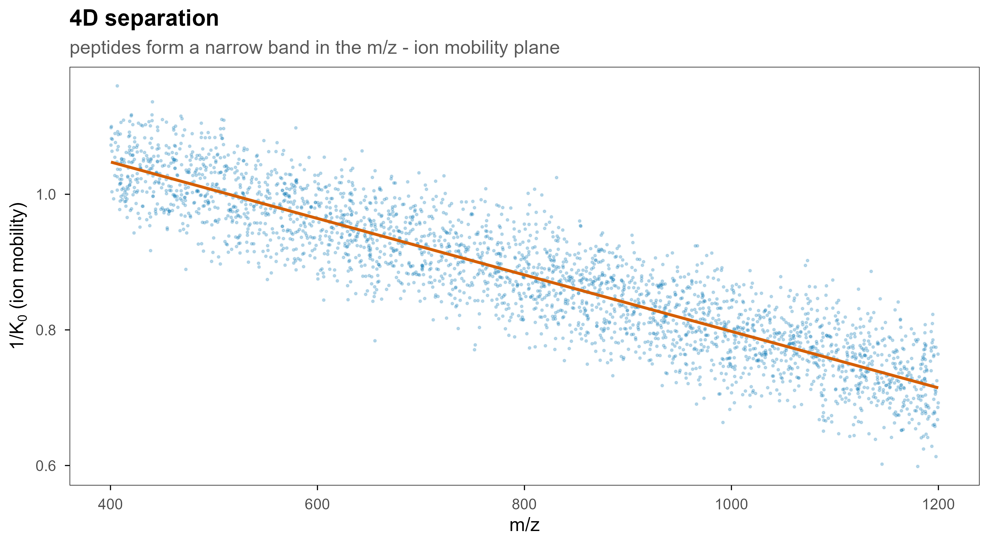
• 离子淌度（ion mobility）在 m/z 和强度之外再加一维：碰撞截面积（CCS）或 1/K0。timsTOF 的 .d 文件因此是 4D 的。
• 碎裂方式决定谱图长什么样：HCD/CID 主要产生 b/y 离子，ETD 对磷酸化和大肽段更友好。

set.seed(3)
n <- 3000
mz <- runif(n, 400, 1200)
k0 <- 1.05 - 0.00042 * (mz - 400) + rnorm(n, 0, 0.045)
ccs_df <- data.frame(mz = mz, k0 = k0)

ggplot(ccs_df, aes(mz, k0)) +
  geom_point(colour = blog_pal[["blue"]], size = 0.35, alpha = 0.22) +
  geom_smooth(method = "lm", formula = y ~ x, colour = blog_pal[["vermillion"]],
              linewidth = 0.8, se = FALSE) +
  labs(
    x = "m/z", y = expression("1/"*K[0]~"(ion mobility)"),
    title = "4D separation",
    subtitle = "peptides form a narrow band in the m/z - ion mobility plane"
  )

Figure 3: 加上离子淌度后，数据从 3D 变成 4D。同一 m/z 上的共洗脱肽段可以在淌度维度被分开，这也是 timsTOF 和 FAIMS 提高鉴定数的核心原因。

3. 一次运行在文件里长什么样

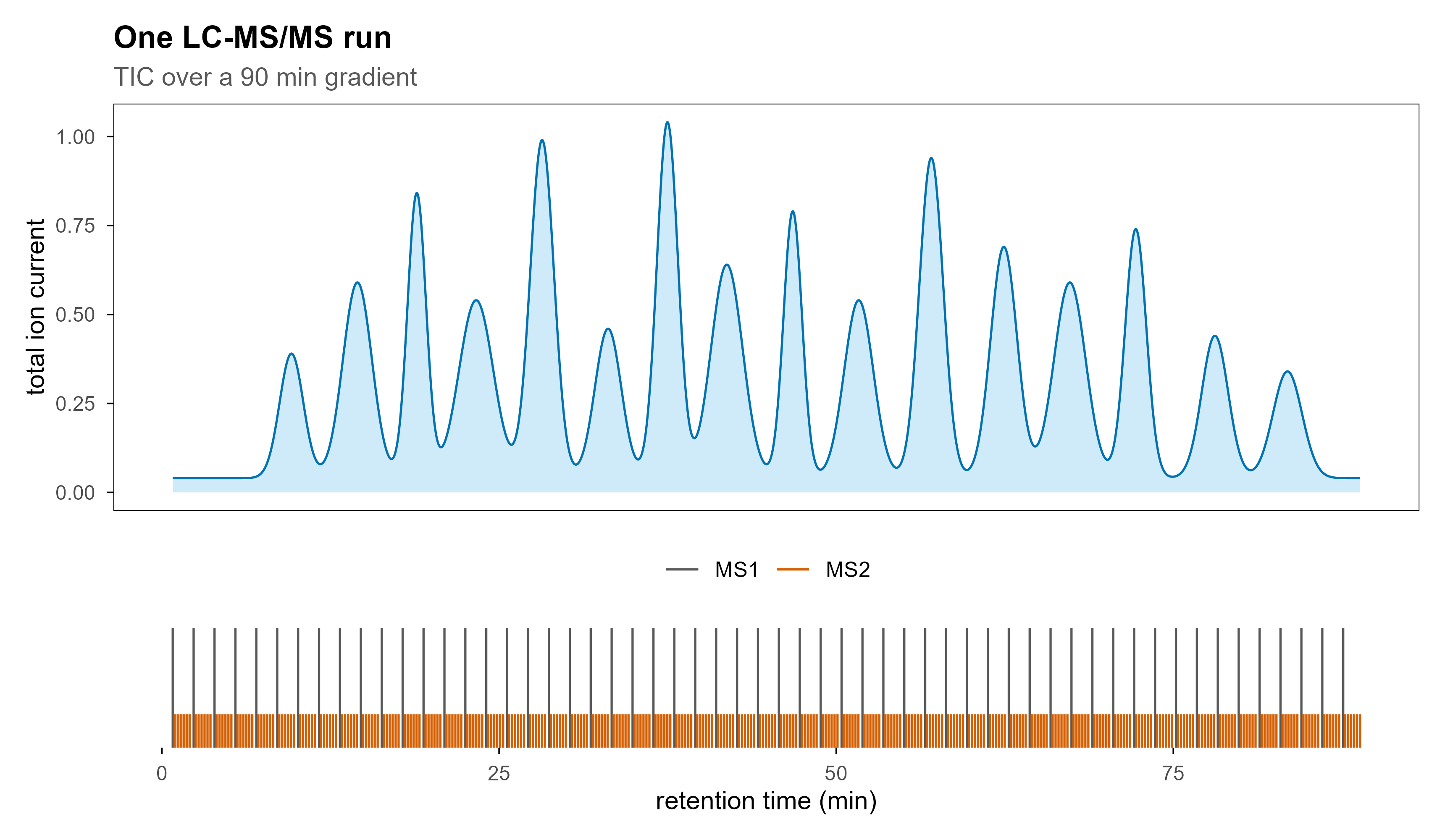
一次 90 分钟的 DDA 运行，典型会产生 3,000–10,000 张 MS1 谱和 30,000–150,000 张 MS2 谱，文件大小从几百 MB 到几 GB。这个规模决定了三件事：不能一次全读进内存、必须能随机访问某一条扫描、必须有索引。

最直观的视图是总离子流（TIC）：把每一张 MS1 谱的所有强度加起来，对保留时间作图。

rt <- seq(0, 90, length.out = 4000)
mu  <- c(9, 14, 18.5, 23, 28, 33, 37.5, 42, 47, 52, 57.5, 63, 68, 73, 79, 84.5)
amp <- c(0.35, 0.55, 0.80, 0.50, 0.95, 0.42, 1.00, 0.60, 0.75, 0.50, 0.90, 0.65, 0.55, 0.70, 0.40, 0.30)
wd  <- c(0.90, 1.10, 0.70, 1.30, 0.90, 1.00, 0.80, 1.20, 0.70, 1.10, 0.90, 1.00, 1.20, 0.80, 1.00, 1.10)

tic <- rowSums(sapply(seq_along(mu), function(i) amp[i] * exp(-((rt - mu[i])^2) / (2 * wd[i]^2))))
tic_df <- data.frame(rt = rt, intensity = tic + 0.04)

p_tic <- ggplot(tic_df, aes(rt, intensity)) +
  geom_area(fill = blog_pal[["sky"]], alpha = 0.28) +
  geom_line(colour = blog_pal[["blue"]], linewidth = 0.45) +
  labs(
    x = NULL, y = "total ion current",
    title = "One LC-MS/MS run",
    subtitle = "TIC over a 90 min gradient"
  ) +
  theme(axis.text.x = element_blank(), axis.ticks.x = element_blank())

cyc <- seq(0.8, 89, by = 1.55)
scan_df <- bind_rows(
  data.frame(t = cyc, level = "MS1", h = 1),
  data.frame(t = as.vector(outer(cyc, seq(0.15, 1.25, length.out = 6), "+")),
             level = "MS2", h = 0.28)
)

p_scan <- ggplot(scan_df, aes(x = t, xend = t, y = 0, yend = h, colour = level)) +
  geom_segment(linewidth = 0.45) +
  scale_colour_manual(values = c(MS1 = "grey35", MS2 = blog_pal[["vermillion"]])) +
  scale_y_continuous(expand = c(0, 0)) +
  labs(x = "retention time (min)", y = NULL, colour = NULL) +
  theme(
    axis.text.y = element_blank(), axis.ticks.y = element_blank(),
    legend.position = "top", panel.border = element_blank()
  )

p_tic / p_scan + plot_layout(heights = c(3.4, 1))

Figure 4: 上：总离子流色谱图，峰是随梯度洗脱出来的肽段群体。下：同一条时间轴上的扫描类型，灰色是 MS1 调查扫描，红色是随后触发的 MS2 碎裂扫描。

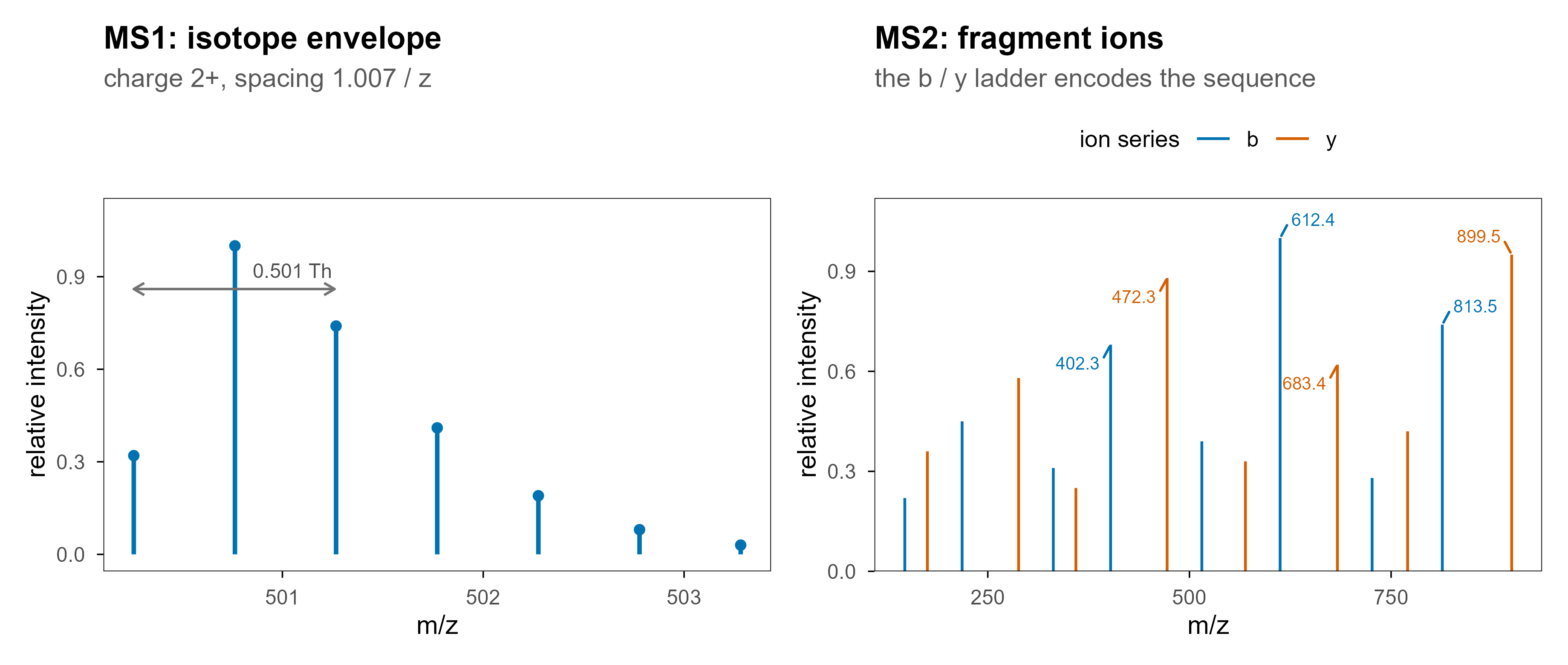
单张谱图则是另一个视图：横轴 m/z，纵轴强度。MS1 上看到的是同位素包络（isotope envelope），MS2 上看到的是碎片离子。

iso <- data.frame(
  mz = 500.26 + (0:6) * (1.00728 / 2),
  intensity = c(0.32, 1.00, 0.74, 0.41, 0.19, 0.08, 0.03)
)
p_ms1 <- ggplot(iso, aes(mz, intensity)) +
  geom_segment(aes(xend = mz, y = 0, yend = intensity),
               colour = blog_pal[["blue"]], linewidth = 0.9) +
  geom_point(colour = blog_pal[["blue"]], size = 1.6) +
  annotate("text", x = 501.05, y = 0.92, label = "0.501 Th", size = 3, colour = "grey30") +
  annotate("segment", x = 500.26, xend = 501.26, y = 0.86, yend = 0.86,
           arrow = arrow(ends = "both", length = unit(1.8, "mm")), colour = "grey45") +
  labs(x = "m/z", y = "relative intensity", title = "MS1: isotope envelope",
       subtitle = "charge 2+, spacing 1.007 / z") +
  ylim(0, 1.1)

frag <- data.frame(
  mz = c(147.11, 218.15, 331.23, 402.27, 515.35, 612.41, 726.45, 813.48,
         175.12, 288.20, 359.25, 472.33, 569.39, 683.43, 770.47, 899.51),
  intensity = c(0.22, 0.45, 0.31, 0.68, 0.39, 1.00, 0.28, 0.74,
                0.36, 0.58, 0.25, 0.88, 0.33, 0.62, 0.42, 0.95),
  series = c(rep("b", 8), rep("y", 8))
)
lab <- frag %>% filter(intensity > 0.6)

p_ms2 <- ggplot(frag, aes(mz, intensity, colour = series)) +
  geom_segment(aes(xend = mz, y = 0, yend = intensity), linewidth = 0.55) +
  geom_text_repel(
    data = lab, aes(label = sprintf("%.1f", mz)), size = 2.6,
    min.segment.length = 0, box.padding = 0.3, seed = 2,
    max.overlaps = Inf, show.legend = FALSE
  ) +
  scale_colour_manual(values = c(b = blog_pal[["blue"]], y = blog_pal[["vermillion"]])) +
  scale_y_continuous(expand = expansion(mult = c(0, 0.12))) +
  labs(x = "m/z", y = "relative intensity", colour = "ion series",
       title = "MS2: fragment ions", subtitle = "the b / y ladder encodes the sequence") +
  theme(legend.position = "top")

p_ms1 | p_ms2

Figure 5: 左：一个 2+ 肽段在 MS1 上的同位素包络，相邻峰间隔约 0.5 Th，由此可以读出电荷态。右：同一条肽段在 MS2 上的碎片离子，b 与 y 系列拼起来就是序列。

4. DDA、DIA、PRM：三种采集策略

数据长什么样，首先取决于仪器怎么选前体。

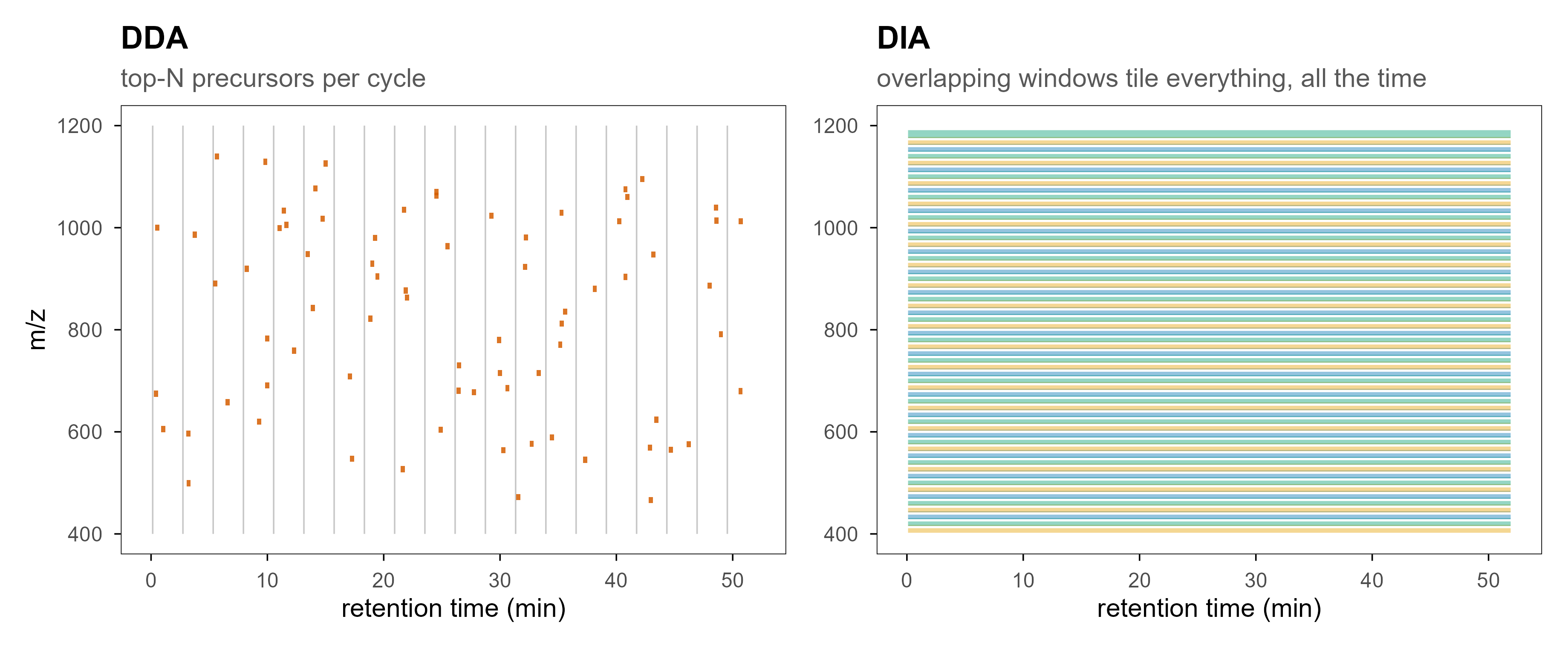
DDA（data-dependent acquisition）：先做一张 MS1 调查扫描，挑信号最强的前 N 个前体，逐个隔离、碎裂、采集 MS2。优点是谱图干净、好搜库；缺点是随机性——强弱共洗脱时弱信号会被挤掉，低丰度肽段在不同重复之间可能时有时无，这就是定量缺失值的主要来源之一。

DIA（data-independent acquisition）：不等选择，按 m/z 切成若干窗口，每个窗口内的所有前体一起碎裂、一起采集。覆盖更稳定、重复性更好；代价是 MS2 谱是混合谱，必须靠谱图库或伪谱库去卷积。

PRM（parallel reaction monitoring）：事先指定目标肽段，把它们的前体列进包含列表，长时间累积信号。这是靶向定量，灵敏度最高，但只能测你列出来的东西。

set.seed(7)
cycles <- 20
ms2 <- do.call(rbind, lapply(seq_len(cycles), function(i) {
  k <- sample(2:5, 1)
  data.frame(
    rt = (i - 1) * 2.6 + runif(k, 0.3, 2.2),
    mz = runif(k, 430, 1150)
  )
}))

p_dda <- ggplot() +
  geom_segment(
    data = data.frame(rt = (seq_len(cycles) - 1) * 2.6 + 0.14),
    aes(x = rt, xend = rt, y = 400, yend = 1200),
    colour = "grey78", linewidth = 0.3
  ) +
  geom_rect(
    data = ms2,
    aes(xmin = rt - 0.18, xmax = rt + 0.18, ymin = mz - 6, ymax = mz + 6),
    fill = blog_pal[["vermillion"]], alpha = 0.85
  ) +
  coord_cartesian(xlim = c(0, 52), ylim = c(400, 1200)) +
  labs(x = "retention time (min)", y = "m/z", title = "DDA",
       subtitle = "top-N precursors per cycle") +
  theme(legend.position = "none")

w <- 20
starts <- seq(400, 1200 - w, by = w * 2 / 3)
dia <- data.frame(ymin = starts, ymax = starts + w, idx = seq_along(starts))

p_dia <- ggplot(dia) +
  geom_rect(
    aes(xmin = 0, xmax = 52, ymin = ymin, ymax = ymax, fill = factor(idx %% 3)),
    colour = "white", linewidth = 0.45, alpha = 0.42
  ) +
  scale_fill_manual(values = pal[c(1, 5, 3)], guide = "none") +
  coord_cartesian(xlim = c(0, 52), ylim = c(400, 1200)) +
  labs(x = "retention time (min)", y = NULL, title = "DIA",
       subtitle = "overlapping windows tile everything, all the time") +
  theme(legend.position = "none")

p_dda | p_dia

Figure 6: 左：DDA 只碎裂被选中的前体，取样是稀疏且随机的。右：DIA 用相互重叠的窗口铺满整个 m/z 范围，取样是系统性的。

维度	DDA	DIA	PRM
前体选择	实时、依赖强度	无选择，窗口内全采	事先指定
谱图内容	单前体（近似）	多前体混合	单前体、长时间累积
缺失值	较多（随机漏采）	少（系统性覆盖）	只针对目标肽段
数据分析	直接搜库	谱图库 / 伪谱库 / 去卷积	提取离子色谱
典型用途	发现型研究	大队列定量	验证与临床检测

5. 原始数据格式的架构

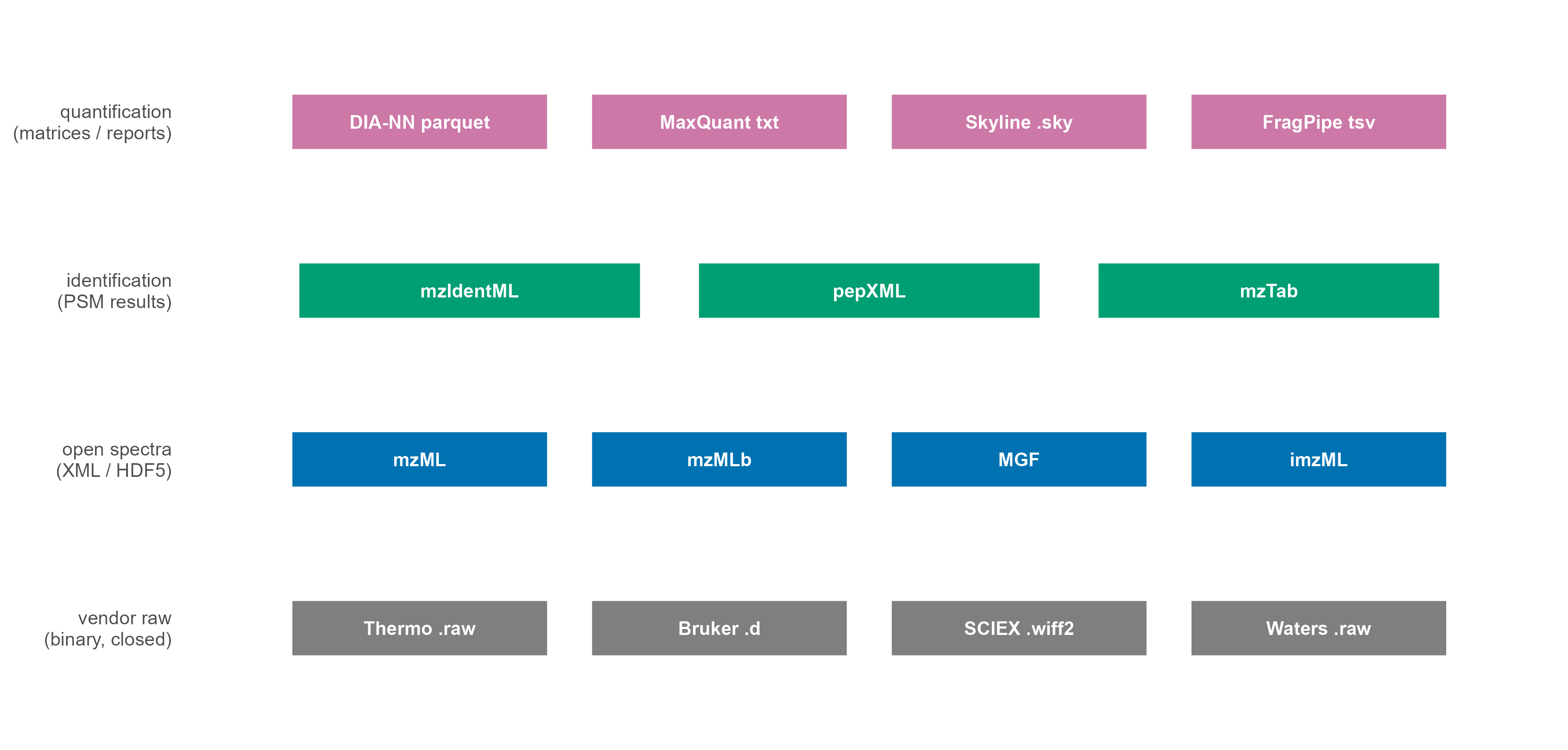
这是本文的核心部分。理解格式的关键，是把文件分成四层：

1. 厂商原始层：仪器直接写出的文件，包含完整扫描信息，但二进制结构不公开。
2. 开放谱图层：把原始层无损转换成语义明确的谱图格式，主要是 mzML。
3. 鉴定结果层：搜库软件输出的 PSM / peptide / protein 记录（mzIdentML、pepXML、mzTab）。
4. 定量与处理层：矩阵、报告表、项目文件（parquet、TSV、Skyline .sky、FragPipe 输出等）。

fmt <- data.frame(
  layer = factor(
    c(rep("vendor raw", 4), rep("open spectra", 4), rep("identification", 3), rep("quantification", 4)),
    levels = c("vendor raw", "open spectra", "identification", "quantification")
  ),
  name = c(
    "Thermo .raw", "Bruker .d", "SCIEX .wiff2", "Waters .raw",
    "mzML", "mzMLb", "MGF", "imzML",
    "mzIdentML", "pepXML", "mzTab",
    "DIA-NN parquet", "MaxQuant txt", "Skyline .sky", "FragPipe tsv"
  )
) %>%
  group_by(layer) %>%
  mutate(pos = row_number(), n = n()) %>%
  ungroup() %>%
  mutate(
    x = (pos - 0.5) / n,
    y = as.numeric(layer),
    half = 0.43 / n
  )

ggplot(fmt) +
  geom_rect(
    aes(xmin = x - half, xmax = x + half, ymin = y - 0.17, ymax = y + 0.17, fill = layer),
    colour = "white", linewidth = 0.6
  ) +
  geom_text(aes(x, y, label = name), size = 2.8, colour = "white", fontface = "bold") +
  scale_fill_manual(
    values = c("vendor raw" = blog_pal[["grey"]], "open spectra" = blog_pal[["blue"]],
               "identification" = blog_pal[["green"]], "quantification" = blog_pal[["purple"]]),
    guide = "none"
  ) +
  scale_y_continuous(
    breaks = 1:4,
    labels = c("vendor raw\n(binary, closed)", "open spectra\n(XML / HDF5)",
               "identification\n(PSM results)", "quantification\n(matrices / reports)"),
    limits = c(0.55, 4.45)
  ) +
  coord_cartesian(xlim = c(-0.02, 1.02), clip = "off") +
  labs(x = NULL, y = NULL) +
  theme_blog() +
  theme(
    axis.text.x = element_blank(), axis.ticks = element_blank(),
    panel.border = element_blank(), legend.position = "none",
    axis.text.y = element_text(size = 8, lineheight = 0.95)
  )

Figure 7: 四层格式的分工。分析代码通常只和上面三层打交道，但排错时必须回到最底层的原始文件。

5.1 厂商封闭格式

平台	扩展名	实际结构	说明
Thermo Fisher（Orbitrap、Astral、TSQ）	.raw	单文件，内部是扫描头 + 二进制数组	最常见；读取需要官方 RawFileReader 或先转换
Bruker（timsTOF、maXis）	.d	目录，含 analysis.tdf、analysis.tdf_bin、*.baf	4D 数据（含离子淌度），几乎必须先用厂商 SDK 或 alphatims
SCIEX（TripleTOF、ZenoTOF）	.wiff + .wiff.scan，或 .wiff2	元数据与扫描数据分离（新版合并）	转换前务必两个文件放一起
Agilent（Q-TOF、6545）	.d	目录，AcqData/*.bin	MassHunter 结构
Waters（Synapt、Xevo）	.raw（目录）	目录，MassLynx 内部结构	与 Thermo 的 .raw 同名但完全不同

封闭格式的共同问题：

• 不可逆：一旦厂商停止维护解析库，旧数据就可能读不出来；
• 平台绑定：想批量处理只能装对应 SDK，Windows/Linux 支持不一致；
• 仓库不友好：大二进制 + 目录结构，做版本管理几乎不可能。

所以几乎所有正式的蛋白质组学流程都会做一步”转换一次，之后只读开放格式”。常用转换器是 ProteoWizard 的 msconvert 和 Thermo 官方的 ThermoRawFileParser。

5.2 mzML：开放谱图格式的事实标准

mzML 由 HUPO-PSI 维护，本质是一个 XML 索引 + base64 编码的压缩二进制数组。一个最小的结构如下：

<indexedmzML>
  <mzML version="1.1.0">
    <cvList>            <!-- 受控词表：PSI-MS、UO、MS -->
    <fileDescription>   <!-- 文件内容、来源 -->
    <softwareList>      <!-- 写入该文件的软件与版本 -->
    <instrumentConfigurationList>
    <dataProcessingList>
    <run id="run1" startTimeStamp="...">
      <spectrumList count="84213">
        <spectrum id="controllerType=0 controllerNumber=1 scan=2"
                  index="1" defaultArrayLength="412">
          <cvParam cvRef="MS" accession="MS:1000511" name="ms level" value="1"/>
          <scanList count="1">
            <scan>
              <cvParam accession="MS:1000016" name="scan start time" value="0.0212" unitName="minute"/>
            </scan>
          </scanList>
          <binaryDataArrayList count="2">
            <binaryDataArray>
              <cvParam accession="MS:1000514" name="m/z array" unitName="m/z"/>
              <binary>eJztwTEBAAAAwqD1T20...</binary>   <!-- zlib + base64 -->
            </binaryDataArray>
            <binaryDataArray>
              <cvParam accession="MS:1000515" name="intensity array" unitName="number of detector counts"/>
              <binary>eJztwTEBAAAAwqD1T20...</binary>
            </binaryDataArray>
          </binaryDataArrayList>
        </spectrum>
      </spectrumList>
      <chromatogramList count="3"> ... </chromatogramList>
    </run>
  </mzML>
  <indexList>  <!-- offset 索引，支持随机访问 -->
    <index name="spectrum">
      <offset idRef="...scan=2">12345</offset>
    </index>
  </indexList>
</indexedmzML>

几个容易忽略但很重要的细节：

• 所有字段都由受控词表（CV）定义，例如 MS:1000511 是 ms level，MS:1000514 是 m/z array。这让不同仪器的数据可以语义对齐，也让解析器不必猜字段名。
• 二进制数组是 zlib 压缩后的 base64，通常 32 位 float（m/z 也可以是 64 位 double）。m/z 用 double、intensity 用 float 是最常见的组合。
• indexedmzML 才有索引，未索引的 mzML 只能顺序读，处理大队列时会慢一个量级。
• 谱图顺序是文件顺序，不是 m/z 顺序。很多算法需要先按 m/z 排序，这一步很吃内存。

围绕 mzML 还有几个变体：

格式	载体	适用场景	局限
mzML	XML	通用交换格式，几乎所有工具都支持	文件大、解析慢
mzMLb	HDF5	大文件、需要快速随机访问	工具支持少
MGF	纯文本	只存 MS2 峰，做谱图库、机器学习	丢失 MS1 与大部分元数据
imzML + .ibd	XML + 二进制	质谱成像（MALDI）	只适用于成像数据
mzPeak	列式（parquet 风格）	新提出的高性能开放格式	生态仍在建设中

5.3 鉴定与定量层的格式

搜库之后，数据不再是”谱图”，而是”谱图与肽段的对应关系”：

格式	内容	典型来源
mzIdentML (.mzid)	PSM、肽段、蛋白、打分、FDR、修饰	MS-GF+、Comet、Mascot、MS Amanda
pepXML	每个谱图的候选肽段与打分	TPP、Comet
mzTab	蛋白/肽段层面的汇总表（制表符）	OpenMS、部分流程
MaxQuant msms.txt / proteinGroups.txt	定量 + 鉴定合并表	MaxQuant
report.tsv / report.parquet	前体级定量（DIA）	DIA-NN
.osw	SQLite 结构的 OpenSWATH 结果	OpenSWATH
.sky / .blib	项目文件 / 谱图库	Skyline
combined_protein.tsv	蛋白滚动汇总	FragPipe

5.4 同样的数据，不同的体积

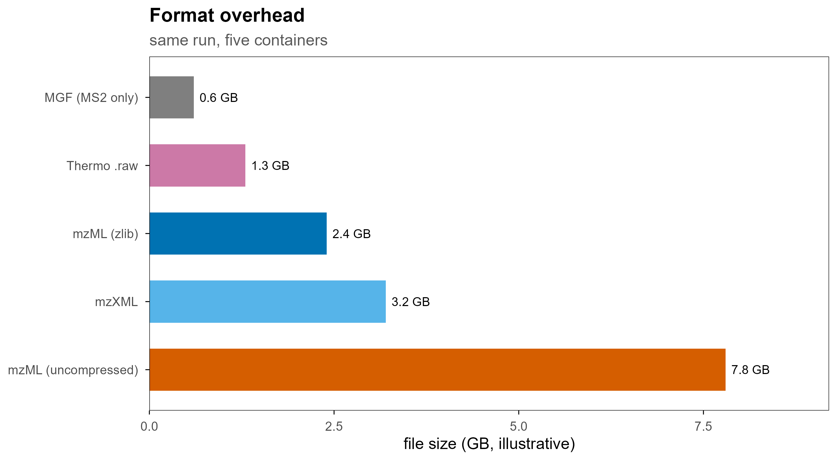
同一次运行转成不同格式，体积差别很大。下面的数字是示意性的量级，不是实测值，但比例关系是真实的：文本格式（MGF）只保留 MS2 所以最小；mzML 不做压缩会膨胀数倍；HDF5 类格式介于两者之间。

sizes <- data.frame(
  format = factor(
    c("MGF (MS2 only)", "Thermo .raw", "mzML (zlib)", "mzXML", "mzML (uncompressed)"),
    levels = rev(c("MGF (MS2 only)", "Thermo .raw", "mzML (zlib)", "mzXML", "mzML (uncompressed)"))
  ),
  gb = c(0.6, 1.3, 2.4, 3.2, 7.8)
)

ggplot(sizes, aes(gb, format, fill = format)) +
  geom_col(width = 0.62, show.legend = FALSE) +
  geom_text(aes(label = paste0(gb, " GB")), hjust = -0.15, size = 3) +
  scale_fill_manual(values = c(
    "MGF (MS2 only)" = blog_pal[["grey"]], "Thermo .raw" = blog_pal[["purple"]],
    "mzML (zlib)" = blog_pal[["blue"]], "mzXML" = blog_pal[["sky"]],
    "mzML (uncompressed)" = blog_pal[["vermillion"]]
  )) +
  scale_x_continuous(limits = c(0, 9.2), expand = c(0, 0)) +
  labs(x = "file size (GB, illustrative)", y = NULL,
       title = "Format overhead", subtitle = "same run, five containers")

Figure 8: 同一次 90 分钟 DDA 运行在不同格式下的示意体积。注意 MGF 体积小是因为它丢掉了 MS1 和大部分元数据，不是因为它更高效。

6. 原始文件里到底存了哪些字段

不管容器是什么，每条扫描通常都带有下列信息。这份清单可以直接用来检查”转换是否丢信息”：

类别	字段	为什么重要
定位	scan number / native ID、index	把 MS2 和触发它的 MS1 关联起来
层级	MS level（1 / 2 / 3）	决定后续处理方式
时间	retention time	色谱对齐、提取离子流
强度	m/z array、intensity array	谱图本体
前体	precursor m/z、charge、单同位素质量	搜库的核心输入
隔离	isolation window 上下界、偏移	DIA 窗口解析必需
碎裂	activation type（HCD/CID/ETD）、碰撞能量	影响谱图可比性
质量	分辨率、质量精度、centroid / profile	决定是否需要 centroiding
淌度	1/K0、CCS、FAIMS CV	4D 数据的第四维
仪器	型号、source、detector、polarity	批次效应排查
汇总	TIC、base peak intensity、injection time、AGC	质控与归一化
色谱	chromatogram list（TIC、BPC、SRM）	快速质控，不必解析全部谱图

一个常见的坑：profile 与 centroid。高分辨仪器原始数据常是 profile（连续采样的峰形），而搜库需要 centroid（峰顶一个 m/z 值）。msconvert 的 --filter "peakPicking true 1-" 就是在做这件事。如果 centroid 参数不合适，同位素峰会被合并或漏掉，直接影响电荷判断。

7. 用 Python 读取

Python 生态里最常用的是 pyteomics（纯 Python、惰性迭代、内存友好）和 pymzml；需要完整工具链时用 pyOpenMS；做谱图相似度与机器学习时用 matchms。

7.1 mzML：流式读取 MS2

from pyteomics import mzml

with mzml.MzML("run.mzML") as reader:
    print(reader.header[:3])          # 软件、仪器等元数据
    for spec in reader:
        if spec["ms level"] != 2:
            continue
        scan = spec["scanList"]["scan"][0]
        rt = scan["scan start time"]   # 默认单位见 unitInfo
        prec = spec["precursorList"]["precursor"][0]
        ion = prec["selectedIonList"]["selectedIon"][0]

        mz = spec["m/z array"]
        intensity = spec["intensity array"]
        print(spec["id"], rt, ion.get("selected ion m/z"),
              ion.get("charge state"), mz[:3], intensity[:3])
        break

要点：

• mzml.MzML 是迭代器，不会把整个文件读进内存；
• 数组是 numpy.ndarray，可以直接做向量运算；
• 电荷、前体 m/z 等键名不保证存在，用 .get()；
• 如果只关心元数据，reader.get_by_id() 配合索引比顺序遍历快得多。

7.2 其他格式

# pymzml：接口更"对象化"
import pymzml
run = pymzml.run.Reader("run.mzML")
for spec in run:
    if spec.ms_level == 2:
        mz, i = spec.peaks("raw")
        break

# matchms：读成标准化 Spectrum 对象，方便算余弦相似度
from matchms.importing import load_from_mzml
spectra = list(load_from_mzml("run.mzML"))
print(spectra[0].metadata)

# pyOpenMS：完整算法库（峰提取、校正、搜库接口）
import pyopenms as oms
exp = oms.MSExperiment()
oms.MzMLFile().load("run.mzML", exp)
print(exp.getNrSpectra(), exp.getNrChromatograms())

# mzIdentML：读鉴定结果
from pyteomics import mzid
with mzid.MzIdentML("search.mzid") as reader:
    for psm in reader:
        print(psm["spectrumID"], psm["chargeState"], psm["PeptideSequence"])

7.3 厂商格式与衍生格式

# Thermo .raw：官方推荐先转开放格式，一次性成本换来长期可复现
# ThermoRawFileParser -i run.raw -o out/ -f 2      (-f 2 = mzML)

# Bruker timsTOF 的 4D 数据
from alphatims.bruker import TimsTOF
data = TimsTOF("run.d", use_bruker_sdk=False)
print(data.shape)          # 语义维度：frame / scan / tof ...

# DIA-NN 的 parquet 报告：列式存储，读取和筛选都快
import pyarrow.parquet as pq
df = pq.read_table("report.parquet").to_pandas()
df = df[df["Q.Value"] <= 0.01]

8. 用 R 读取

R 侧的现代入口是 Spectra（统一的谱图容器，后端可换）。旧的 mzR 仍然可用，很多流程还在用；Thermo 的 .raw 可以直接用 rawrr 读，不必先转换。

8.1 Spectra：推荐方式

library(Spectra)

sp <- Spectra("run.mzML", source = MsBackendMzR())
sp

# 可用的谱图级变量
spectraVariables(sp)

# 常用操作
ms2 <- filterMsLevel(sp, 2L)
ms2 <- filterRt(ms2, c(600, 3600))            # 秒
ms2 <- filterPrecursorMz(ms2, c(400, 1200))
length(ms2)

# 峰数据：每个元素是一个两列矩阵（m/z, intensity）
peaksData(ms2[1:3])

# 元数据表
as.data.frame(spectraData(ms2[1:5], c("spectrumId", "rtime", "precursorMz", "precursorCharge")))

Spectra 的价值在于后端可替换：同一套代码可以读 mzML、MGF、Thermo .raw，甚至换成 SQLite / parquet 后端来处理超过内存的数据集。

# 只含 MS2 的轻量格式
sp_mgf <- Spectra("library.mgf", source = MsBackendMgf())

# 大文件：先落到数据库后端，再按需查询
# sp_db <- Spectra("run.mzML", source = MsBackendMzR())
# sp_db <- setBackend(sp_db, MsBackendSql())

8.2 mzR：老牌底层接口

library(mzR)

f <- openMSfile("run.mzML")
hdr <- header(f)
head(hdr[, c("seqNum", "msLevel", "rtime", "precursorMZ",
             "precursorCharge", "totIonCurrent", "peaksCount")])

pk <- peaks(f, scan = 42)     # 单张谱图：m/z + intensity 两列
chrom <- chromatograms(f)
close(f)

mzR 返回的是扁平数据框，很适合快速探索和质控；缺点是它不理解”谱图集合”这个概念，批量操作要自己写循环。

8.3 直接读 Thermo .raw

library(rawrr)

idx <- readIndex("run.raw")
head(idx)

sp <- readSpectrum("run.raw", scan = idx$scanNumber[1:5])
str(sp[[1]])          # scan header + mZ / intensity

rawrr 通过 Thermo 的 RawFileReader 工作，因此只能在 Windows / Linux 的对应运行时下使用，并且受厂商许可约束。

8.4 鉴定与定量结果

library(PSMatch)

psm <- readMzId("search.mzid")
head(psm)

# 过滤到 1% FDR
psm_f <- filterFdr(psm, fdr = 0.01, keep = TRUE)
table(psm_f$decoy)

library(QFeatures)

# 从 PSM 到 peptide 再到 protein 的聚合容器
qf <- QFeatures(list(psms = psm_assays, peptides = peptide_assays,
                     proteins = protein_assays))
qf <- aggregateFeatures(qf, i = "peptides", fcol = "Protein",
                        name = "proteins_agg", fun = colSums)

下游的差异分析通常接 limma、DEP 或 MSstats；DIA 数据常用 MSstats、DIA-NN 的 R 包或 Spectronaut 导出的矩阵。

9. 从谱图到蛋白表

读取只是第一步。真正决定结果质量的是中间这几步。

9.1 搜库与 FDR

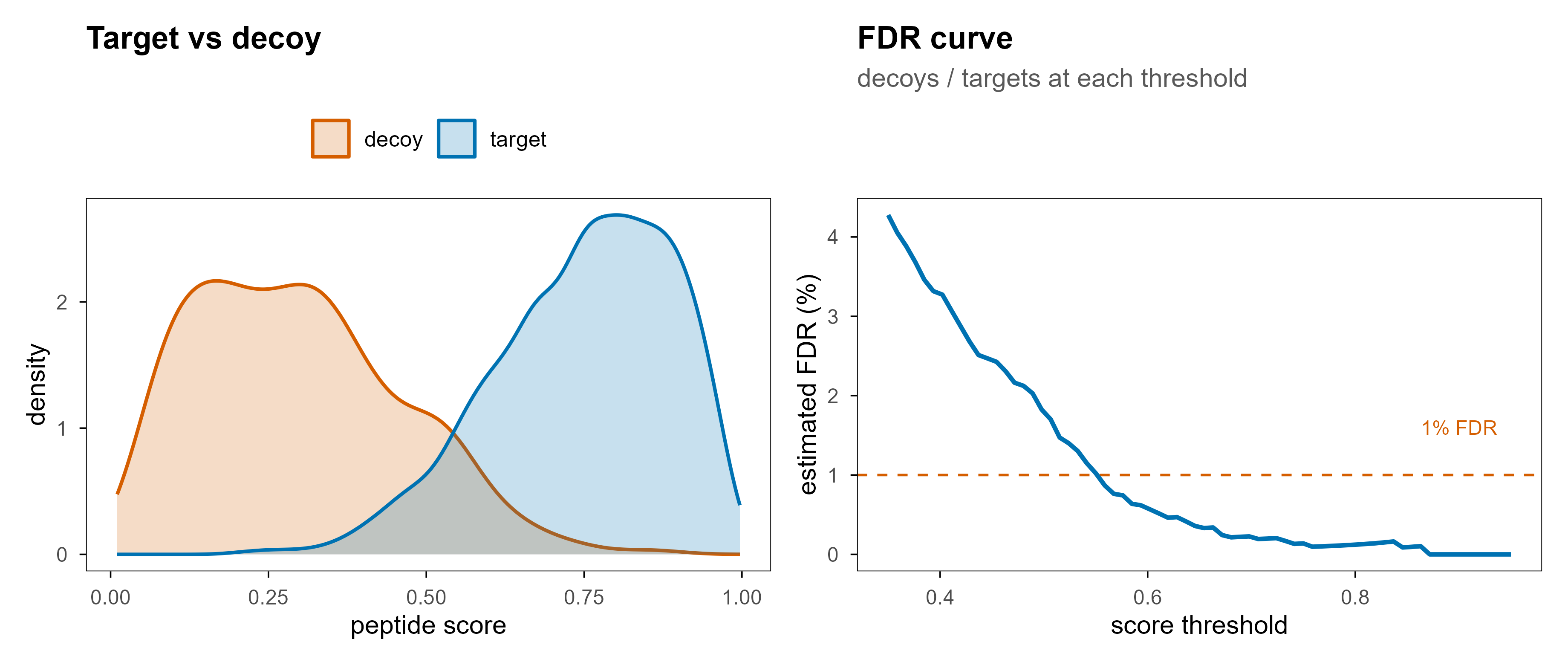
搜库的本质是：给定一张 MS2 谱图和前体质量，在理论酶切肽段库里找最匹配的序列，并给出打分。为了让”匹配”有统计意义，业界通用 target-decoy 策略：把真实库和反转/打乱的诱饵库一起搜，用诱饵命中数估计假阳性。

set.seed(11)
target <- rbeta(4000, 6, 2)
decoy  <- rbeta(500, 2, 5)
score_df <- bind_rows(
  data.frame(score = target, type = "target"),
  data.frame(score = decoy, type = "decoy")
)

p_dens <- ggplot(score_df, aes(score, fill = type, colour = type)) +
  geom_density(alpha = 0.22, linewidth = 0.7, adjust = 1.1) +
  scale_fill_manual(values = c(target = blog_pal[["blue"]], decoy = blog_pal[["vermillion"]])) +
  scale_colour_manual(values = c(target = blog_pal[["blue"]], decoy = blog_pal[["vermillion"]])) +
  labs(x = "peptide score", y = "density", fill = NULL, colour = NULL,
       title = "Target vs decoy") +
  theme(legend.position = "top")

thr <- seq(0.35, 0.95, length.out = 70)
fdr_df <- data.frame(
  threshold = thr,
  fdr = sapply(thr, function(t) sum(decoy >= t) / max(sum(target >= t), 1)) * 100
)

p_fdr <- ggplot(fdr_df, aes(threshold, fdr)) +
  geom_hline(yintercept = 1, linetype = "dashed", colour = blog_pal[["vermillion"]], linewidth = 0.5) +
  geom_line(colour = blog_pal[["blue"]], linewidth = 0.9) +
  annotate("text", x = 0.9, y = 1.6, label = "1% FDR", size = 3,
           colour = blog_pal[["vermillion"]]) +
  labs(x = "score threshold", y = "estimated FDR (%)",
       title = "FDR curve", subtitle = "decoys / targets at each threshold") +
  theme(legend.position = "none")

p_dens | p_fdr

Figure 9: 左：target 与 decoy 的打分分布，decoy 整体偏低。右：随打分阈值变化的估计 FDR，1% 处对应的就是常用的过滤线。

需要注意的几个细节：

• FDR 可以是在 PSM、peptide、protein 三个层级上控制的，数值不可互换；
• 蛋白层面的 FDR 不等于 PSM 层面的 FDR，蛋白推断需要单独的模型（如 picked-protein、hierarchical）；
• 修饰位点还需要定位概率（localization probability），否则会把”有修饰”和”修饰在哪个残基”混为一谈。

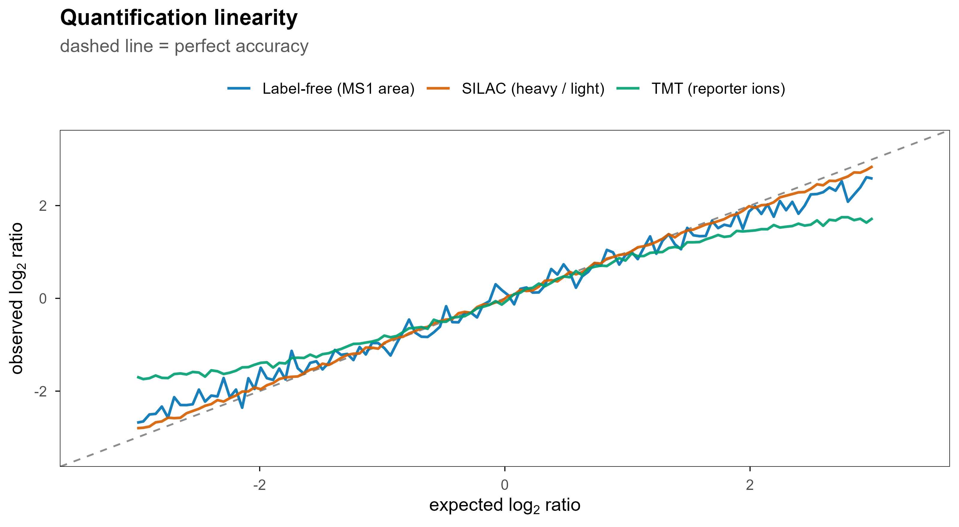
9.2 四条定量路线

策略	原理	优点	局限
Label-free（LFQ）	比较同一肽段在不同运行中的 MS1 峰面积	成本低、样本数不受限	运行间波动大，缺失值多
同重标（TMT / iTRAQ）	不同样本标记后混样，MS2 里读报告离子	多重、通量高、缺失少	比值压缩（ratio compression）
代谢标（SILAC）	轻重同位素培养，混样后成对出现	定量最准	只能用于可培养细胞
DIA 定量	从混合 MS2 中提取前体色谱	覆盖稳定、重复性好	依赖谱图库质量

x <- seq(-3, 3, length.out = 120)
set.seed(9)
quant_df <- bind_rows(
  data.frame(expected = x, observed = x * (1 - 0.05 * abs(x)) + rnorm(length(x), 0, 0.17),
             method = "Label-free (MS1 area)"),
  data.frame(expected = x, observed = x * (1 - 0.14 * abs(x)) + rnorm(length(x), 0, 0.04),
             method = "TMT (reporter ions)"),
  data.frame(expected = x, observed = x * (1 - 0.02 * abs(x)) + rnorm(length(x), 0, 0.03),
             method = "SILAC (heavy / light)")
)

ggplot(quant_df, aes(expected, observed, colour = method)) +
  geom_abline(slope = 1, intercept = 0, linetype = "dashed", colour = "grey55") +
  geom_line(linewidth = 0.75, alpha = 0.9) +
  scale_colour_manual(values = pal[c(1, 2, 3)]) +
  coord_cartesian(xlim = c(-3.3, 3.3), ylim = c(-3.3, 3.3)) +
  labs(x = expression("expected "*log[2]*" ratio"), y = expression("observed "*log[2]*" ratio"),
       colour = NULL, title = "Quantification linearity",
       subtitle = "dashed line = perfect accuracy") +
  theme(legend.position = "top")

Figure 10: 三种策略的定量线性度示意。同重标在高比值端会出现明显压缩，代谢标最接近理想直线，label-free 噪声最大。

9.3 缺失值不是随机的

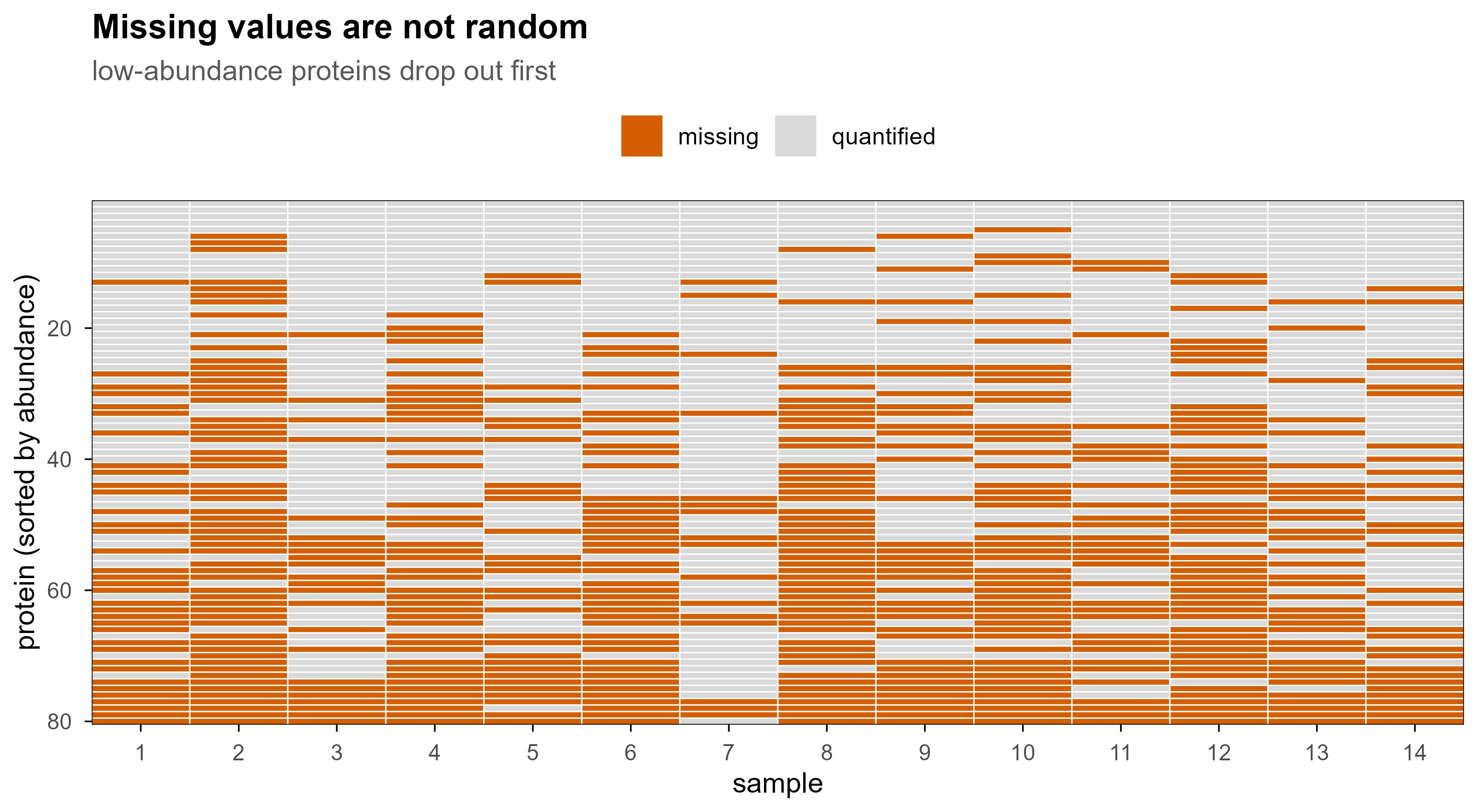
蛋白质组数据里的缺失值主要有三种来源：低于检测限（MNAR）、DDA 随机漏采、以及数据处理过滤。绝大多数情况下，缺失与丰度相关，所以”用 0 填补”或”用均值填补”都会系统性扭曲结果。

set.seed(5)
n_prot <- 80
n_smp <- 14
base <- sort(rnorm(n_prot, 0, 1), decreasing = TRUE)
mat <- outer(base, rnorm(n_smp, 0, 0.55), "+")
p_miss <- plogis(-mat * 1.5)
miss <- matrix(runif(n_prot * n_smp) < p_miss, n_prot, n_smp)

miss_df <- expand.grid(protein = 1:n_prot, sample = 1:n_smp)
miss_df$status <- ifelse(as.vector(miss), "missing", "quantified")

ggplot(miss_df, aes(sample, protein, fill = status)) +
  geom_tile(colour = "white", linewidth = 0.25) +
  scale_fill_manual(values = c(quantified = "#D9D9D9", missing = blog_pal[["vermillion"]])) +
  scale_y_reverse(expand = c(0, 0)) +
  scale_x_continuous(expand = c(0, 0), breaks = 1:n_smp) +
  labs(x = "sample", y = "protein (sorted by abundance)", fill = NULL,
       title = "Missing values are not random",
       subtitle = "low-abundance proteins drop out first")

Figure 11: 低丰度蛋白优先缺失（MNAR）。这类矩阵不能用简单的均值或零填补，通常需要过滤、删失模型或专门的归一化方法。

常用的处理路线：

• 过滤：要求至少在 70% 的样本中被定量（大队列里更常见）；
• 删失模型：MSstats、DEqMS 的思路，把缺失当作”低于检测限”而不是随机缺失；
• 归一化：中位数、quantile、vsn、或基于内参/峰面积总和；
• 批次校正：limma::removeBatchEffect、ComBat，但必须在建模时保留批次因子。

10. 基于质谱之外，还有哪些蛋白质组学方法

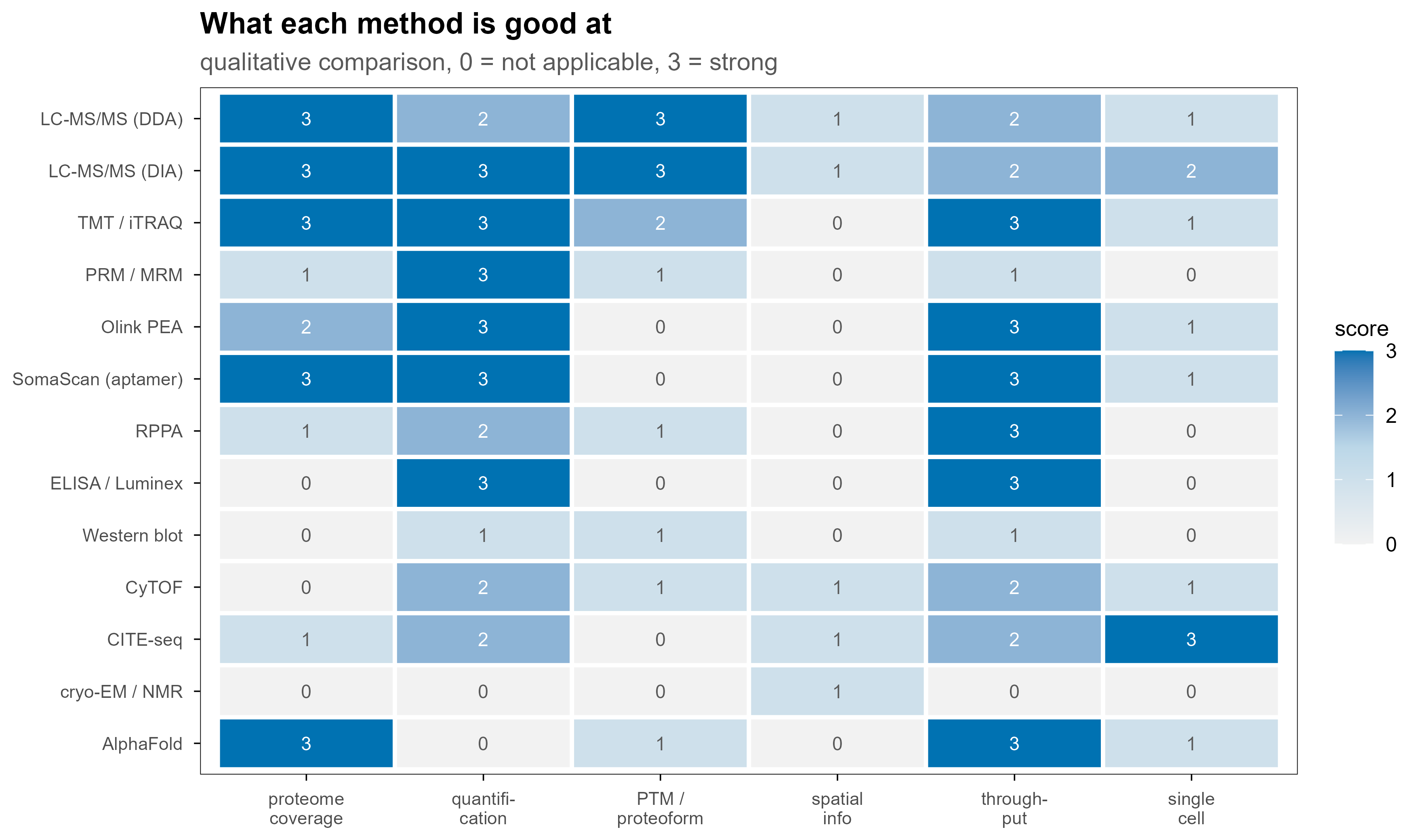
质谱不是唯一路线。不同方法在”覆盖广度、定量精度、空间信息、通量”上各有取舍，实际研究里常常是组合使用。

cap <- data.frame(
  method = c(
    "LC-MS/MS (DDA)", "LC-MS/MS (DIA)", "TMT / iTRAQ", "PRM / MRM",
    "Olink PEA", "SomaScan (aptamer)", "RPPA", "ELISA / Luminex",
    "Western blot", "CyTOF", "CITE-seq", "cryo-EM / NMR", "AlphaFold"
  ),
  coverage       = c(3, 3, 3, 1, 2, 3, 1, 0, 0, 0, 1, 0, 3),
  quantification = c(2, 3, 3, 3, 3, 3, 2, 3, 1, 2, 2, 0, 0),
  PTM            = c(3, 3, 2, 1, 0, 0, 1, 0, 1, 1, 0, 0, 1),
  spatial        = c(1, 1, 0, 0, 0, 0, 0, 0, 0, 1, 1, 1, 0),
  throughput     = c(2, 2, 3, 1, 3, 3, 3, 3, 1, 2, 2, 0, 3),
  single_cell    = c(1, 2, 1, 0, 1, 1, 0, 0, 0, 1, 3, 0, 1)
) %>%
  pivot_longer(-method, names_to = "dimension", values_to = "score") %>%
  mutate(
    method = factor(method, levels = rev(c(
      "LC-MS/MS (DDA)", "LC-MS/MS (DIA)", "TMT / iTRAQ", "PRM / MRM",
      "Olink PEA", "SomaScan (aptamer)", "RPPA", "ELISA / Luminex",
      "Western blot", "CyTOF", "CITE-seq", "cryo-EM / NMR", "AlphaFold"
    ))),
    dimension = factor(dimension,
      levels = c("coverage", "quantification", "PTM", "spatial", "throughput", "single_cell"),
      labels = c("proteome\ncoverage", "quantifi-\ncation", "PTM /\nproteoform", "spatial\ninfo", "through-\nput", "single\ncell"))
  )

ggplot(cap, aes(dimension, method, fill = score)) +
  geom_tile(colour = "white", linewidth = 0.9) +
  geom_text(aes(label = score, colour = score >= 2), size = 3, show.legend = FALSE) +
  scale_fill_gradientn(colours = c("#F2F2F2", "#BBD7E8", blog_pal[["blue"]]), limits = c(0, 3)) +
  scale_colour_manual(values = c(`TRUE` = "white", `FALSE` = "grey35")) +
  labs(x = NULL, y = NULL, fill = "score",
       title = "What each method is good at",
       subtitle = "qualitative comparison, 0 = not applicable, 3 = strong") +
  theme(
    axis.text.x = element_text(size = 8, lineheight = 0.9),
    axis.text.y = element_text(size = 8),
    legend.position = "right"
  )

Figure 12: 不同蛋白质组学方法的能力画像。分数是定性的（0–3），用于比较方法的相对取舍，不代表任何具体产品的性能。

10.1 亲和与抗体类

这类方法的共同点是用已知的结合试剂识别已知的目标，因此只能测”你已经有试剂的东西”。

• ELISA：单靶标、定量准确、临床金标准，但一次一个蛋白。
• Luminex xMAP：把抗体挂在荧光编码微球上，一次几十个靶标。
• RPPA（反相蛋白阵列）：把样本点成阵列再用抗体探测，适合信号通路蛋白和磷酸化位点，通量高但依赖抗体质量。
• Olink PEA：一对带 DNA 标签的抗体同时结合目标，标签互补后通过 qPCR 或 NGS 读出，双抗体识别显著降低非特异信号；样本量小（µL 级），适合大队列血浆。
• SomaScan：用慢速解离速率（slow off-rate）的 DNA 适配体代替抗体，可覆盖数千种蛋白，但适配体特异性需要交叉验证。

10.2 流式与单细胞

• 流式细胞术：荧光标记抗体，单细胞、多参数，通量极高，但参数受荧光通道限制（通常 10–30 个）。
• CyTOF（质谱流式）：用金属同位素标记抗体，用 ICP-TOF 读出，通道数可到 40–50，几乎没有自发荧光；代价是细胞被破坏、通量低于荧光流式。
• CITE-seq：把抗体偶联到 DNA 条形码上，和单细胞转录组一起测序，实现同一细胞的蛋白 + mRNA 联合测量。
• 单细胞蛋白质组（SCoPE-MS / SCoPE2、nanoPOTS）：质谱路线的单细胞方案，目前每个细胞可鉴定数百到两千个蛋白，仍处于快速发展阶段。

10.3 相互作用与邻近标记

• AP-MS：把诱饵蛋白拉下来，用质谱鉴定共沉淀的伙伴。
• BioID / TurboID / APEX：用工程化酶给邻近蛋白打上生物素标签，再富集鉴定，能捕获弱且瞬时的相互作用。
• 酵母双杂交、噬菌体展示：二元互作的高通量筛选，假阳性/假阴性都较明显。

10.4 结构与计算

• X-ray 晶体学：原子分辨率，但需要结晶。
• cryo-EM：近原子分辨率、不需要结晶，适合大复合物；通量和样品要求仍是门槛。
• NMR：溶液态、可看动态，但分子量上限明显。
• HDX-MS、交联质谱（XL-MS）：质谱路线的结构探针，给出溶剂可及性和距离约束，常与结构预测互补。
• AlphaFold / ESMFold：直接预测结构，覆盖全蛋白组，但不提供丰度、修饰或相互作用信息，也依赖训练集覆盖度。

10.5 一张对照表

方法	一次测多少	定量能力	是否需要抗体/适配体	典型场景
LC-MS/MS（DDA / DIA）	数千到上万蛋白	中—高	否	发现型研究、修饰组学
TMT / iTRAQ	同一批 10–18 个样本	高（多重）	否	大队列、临床样本
PRM / MRM	几十到几百个目标肽段	很高	否	靶向验证
Olink / SomaScan	一千到七千个蛋白	高	是	血浆大队列生物标志物
RPPA	数百个蛋白/位点	中	是	通路与磷酸化
ELISA / Luminex	1 到几十个	很高	是	临床检测
Western blot	1 到几个	低—中	是	验证
CyTOF	单细胞、40+ 参数	中	是	免疫分型
CITE-seq	单细胞、蛋白 + mRNA	中	是	多组学单细胞
cryo-EM / NMR	一个复合物	不适用	否	结构解析
AlphaFold	全蛋白组	不适用	否	结构预测

11. 落地：一条可复现的处理链路

把上面的内容串起来，一条务实的流程大致是：

raw/                     厂商原始文件，只读，永不修改
  2026-10-26_run01.raw
converted/               msconvert 转换一次，之后只读这里
  2026-10-26_run01.mzML
search/                  搜库输出
  run01.mzid
quant/                   定量矩阵
  report.parquet
figures/                 图表

建议的做法：

1. 原始文件只读，所有转换产物单独目录，转换参数写进脚本或 README；
2. 保留 mzML，不要只留 MGF——后面要复查 MS1、同位素或电荷时会用到；
3. 先用质控指标筛运行：TIC 形状、前体质量误差（ppm）、漏切比例、MS2 数量、iRT 稳定性、carryover；
4. 记录软件与版本：搜库引擎、FDR 阈值、定量方法、数据库版本（含 isoform 与 contaminant）；
5. 统计分析前先看缺失模式，再决定过滤与填补策略；
6. 差异分析用能处理缺失与批次的模型：limma + DEqMS / MSstats，而不是简单的 t 检验。

12. 术语表

术语	含义
PSM	peptide-spectrum match，一张谱图与一条肽段的匹配
FDR	false discovery rate，假发现率
precursor	被选中的母离子（肽段离子）
fragment ion	碎裂后产生的离子，主要是 b / y 系列
TIC / BPC	总离子流 / 基峰色谱
centroid / profile	峰顶取单值 / 保留完整峰形
CCS / 1/K0	碰撞截面积 / 离子淌度
LFQ	label-free quantification
TMT / iTRAQ	同重同位素标记试剂
SILAC	细胞培养稳定同位素标记
DDA / DIA / PRM	数据依赖 / 数据独立 / 平行反应监测
MNAR	missing not at random，缺失与数值本身相关
mzML	HUPO-PSI 维护的开放质谱数据格式

13. 参考

• mzML 规范（HUPO-PSI）：https://www.psidev.info/mzml
• ProteoWizard / msconvert：https://proteowizard.sourceforge.io/
• pyteomics 文档：https://pyteomics.readthedocs.io/
• matchms 文档：https://matchms.readthedocs.io/
• Spectra / Bioconductor：https://bioconductor.org/packages/Spectra
• rawrr：https://bioconductor.org/packages/rawrr
• MSnbase / QFeatures：https://bioconductor.org/packages/QFeatures
• DIA-NN：https://github.com/vdemichev/DiaNN
• MaxQuant：https://www.maxquant.org/
• FragPipe：https://fragpipe.nesvilab.org/
• Skyline：https://skyline.ms/
• Olink PEA：https://olink.com/
• SomaLogic SomaScan：https://somalogic.com/